����� ��������� �������� �������� ���, ������ � �������� ��� � ���������. ���� ������ ����, �����, ����� ����, �����, �������� �������, �����, ������� � �������� �������
��� ��, ��������, ��� ������ ���� ���� �� �� ���� ���� ���� Data Science.
� ���������, ���� ����� ���� �������� ����������� ����������� �������� �� �����������, ������� ������ ��������� ������ � ����
��� ���������� ���� �������� ����� � ������ �� ������
����������� ������ �� �
���������� ������ ����, ��� � ����� ����������.
� ������� ���� ������� �� ������ ������ ������������� ���������� ����� �� �� ������� (��
Python �
C# ��������������). � ���� ��� ��������� ������ ������ ������������� ������������ �� �� ������ ���� ����� (�� ���� ����� ������� ��� ������ �� ���).
���� �� ��� �������� ���� ����, �� ����� ����� ������� dataset ��
Github � ���������� � ���� ������� ��������������. � ��� ����, ��� � � �������� ����� ������.
����� ������� � ���� ��� ������ ��������� � ����� ������� �� ������.
����� �������� ������ ���������� �������� ������ � ���������� �������, �� ��� �������� ����� �� ����������� �� ������.
������
�� � �������� ������ �� ������, �� ���� �� ������ ������� � ����� � ������ (Data Science), �� � ������� ��� ��� �� ���������� ������ ������ � ���������� ��������������� �������, ������ ��� ��� � ��������� ���� ������ ���� ������� �� Data Science ������� �������, ���� �� ��� �������� ������ ������� ���� ����, �� � �� ��� �� ���� ��������� ��� �������� � ����� ������� ��� �� �������� ������ ��������. �������, ���� �� ������ ������, ����������, ��� � ������� (� �� ��� ��� �������) �������� ����� ��� � �� �������, ��� �� ����� �� ���� � ��� ���� �������� � �������� ��������� �������� � ������� ������ ������ �������.
����, ��� �������� ������ � ������� ��������� (�� ������ � ���������)
����� �� �������� ���������� � ��������� ������������
GadPetrovich ������� � ���� ������ ���� ������ ���������� � ���������.
����������:
������ I: ������� ������ ��� ��� ��� ������ ���� �� ��� �� ��������� ���� ���������� ���� ������.
������ II: ����� ������ ��� ������, ��� ��� ������ �� ������ ���������� �� �������
������ III: ����� ������ ��� ������� � ���������� ������ ������
������ IV: ����� ������� �� ��, ��� ��� ���������������� ����� � ������
������ V: ������� ������� �������� ���� ��� ������ � ���������� ������ ����� � �����
������ VI: ����������� ������ ��� ���������� ���� ������� ���������� ���-�� �� ���� �������!
������ VII: ����������� ���� � ������ ����������
������
��, ����� ������ ���������, � � ��� �����, ��� ������ ����� � ������ �������������� �����.
����, �������, ���
� ������� ��� �� � ���� ����������� �������: �������� ������ ������������ ������ ������ ��� ������ ��������� ��������, �������� ������� ��������������� ���� ������ �� ������� ������������� ��������� � ���������� ����, � ����� ������������ � ������������� � ������� PCA, T-SNE � DBSCAN.
� ���� ��� ������ ������������ ������� �� ����� ����������, ������ ��������� ����� ��������.
������� ����-���� ������ �����, ��� ��� ���� ����� ������ �� ��������� �� ������ �� ������ �������, � ���� ��� � ������� �� �������� SVC �������������, � ����� �������� �������� � ���, ��� ��������������� �������� ������ ����� ���� ����� ��������.
������
������ � ���� ��� ����� ������ ���� ����� (���)?
�� ��� �������� ��� ���:
��� �� ���� ���� �������� �����������, ��� � ��� ��� ������� ����� � ������ ����� ����� ����� ������ ��� ��� ���� ���� �� ������ ��� ��� (��� � ����� ����� �� �������� ������).
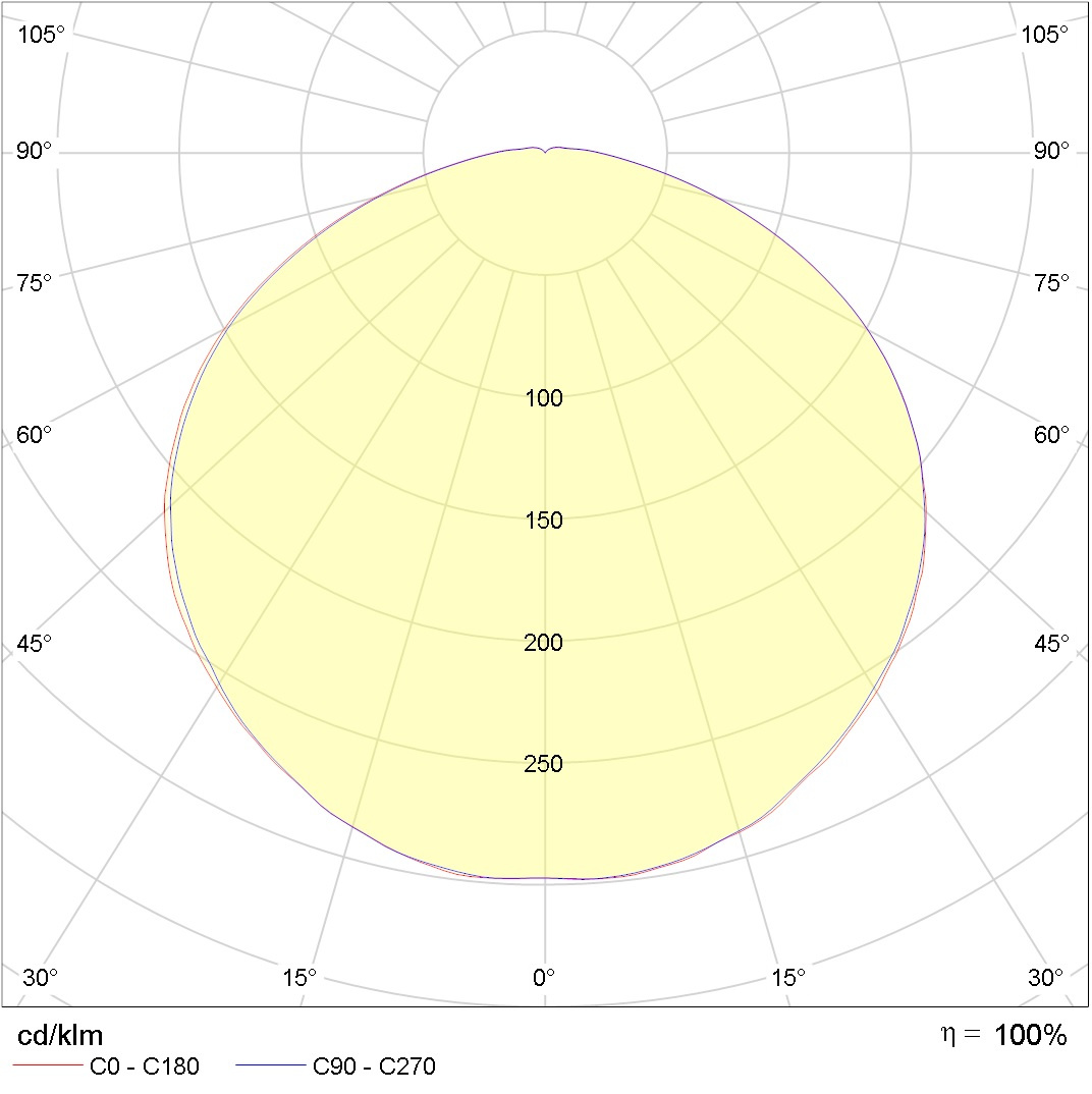
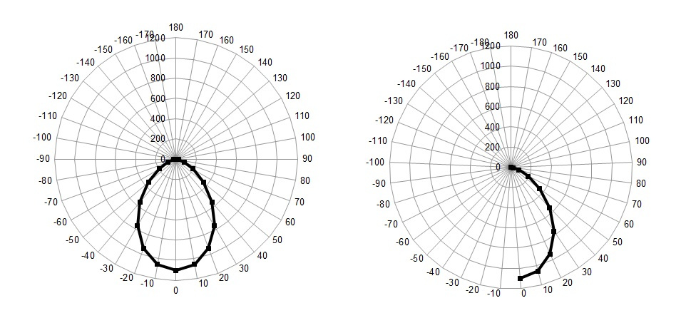
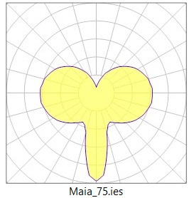
�� ���� �������� �������� ���� ����� (�������� �� ������) � ������ �������� ����� (����������� ��� ��� ���������� ������ ����� �����������), � ������� ���� ������������ ����� 0-180 � 90 � 270 (�����������, ��� ��� ���������� ������ ����� �����������). �������� � �� �����, ����� ��������, �� ������������� � ������ ���������� ���������� � ���������� �� ������������
�������� 833 � �����
�� �������� � �������� ������, �� ������� �� �������, �� ��� �����������, ������� �� ����� ������� ���������������� ����� �� ������ �������������, � ������ ����� �������� ����������. � � ���� ����� �� ������ � ��� ������� �������� ������� �� �� ���������� �� ����������
����� ������ ���? ��� ����� ������, ������ ������������, � ���, ����� ��� ���� ������.
����������� �������� � ��� � .ies ����� ��� ������������ ������ ��� ������� ��� � ��������������� ������� ���������� ������
������� , ����������� ��� ������� �������, ��� ������� �� ���� ���� ������� ������ �� ��������.
�������� ������������ ��������, ��� ���� � �����������, ����� �������� ������ ��� ��� ��� � ������ ������ ���������� ����� ������?
��� �� �������� �����?!
�� ������ ����� ������ ����������� � ���, ��� �� ���������� ������ ��� � ��������� ��� ������, ����� ����������, ����������������, ������������ � ��������� �������� � ������ �� ��� ������������� �������� ��������.
������ ������� �� �������
��� ��� �������� ����������� .ies ����
IESNA:LM-63-1995
������ ������ ������ � ������������� � ����������� ����������, � ����� ��������������� ������ � ����������� � ��� ����� ���� ����� � ����������� �� �������� � ������������ �����, ������ � ������� ��� � �����.
� ����� � ������� ��� ��� 193 �����, � ���� �� � �� ���� ���� �������� ������������ �� � ������.
� ����� ������� ��� ������ ����
���� � ������� �������� ������� ��������� .ies ����� � ������ �������, ������������� ���������� � ������ ������ ������ ��������� ������� ��� � �����, ��� ������ ��� ���� ��������� � ��������� �����.
�� ��� ���, ��� � ������ ��������� ������������� ��� ������� � ������ ���� ��������� ��� ������. ������� �������� � ����������������� �������� ������.
������
����, ������� � �������� ������� � ������� ���������� �� ������� � ���� �������� �� � ���� ������ �� ������, ��� ��� ����, ����� ���������������� ����������� � ����� ������-���������������� �������, ��� ������ ������ ����� ������ ��� �����-�� ����� ������������ ���� � ������ ������ ������ ���� � � ��������� �������� ����� �� 0 �� 180, � ����� 10 (������ ��� ��� ������ ����� �� �������� ��� ������ �� ��������).
�� ���� � ����� ������, ������ ����� ��������� �� ��� �� ������� �����, � ��� �� ������� ������.
������ ���� ��� �� ����, �� � ������� ����������� ��������� � MS Excel, ����� ������ ������� ������� ���.
��������� � ������ �� �������� ���������� ������������ � ������� ��� ������������ ������������, �� ����� � ���� ������������� 4 ����, ������� ������ ����� � �������� ������ ������.
����, � ��� ���� ��������� ���:
����������������� (�), �������� (�), ���������� (�) � ����-������� (�).
�� ���� ����������� ������������ ���� ����� ��������� � ���������� ����� ��������������:
� = 0�-15�; � = 0�-30�; � = 0�-35�; � = 35�-55�;
����� �� � ������ ������ ��������� ���������������
� 1; � = 2; � = 3; � = 4; (���� ���� � ���� ������, �� ������ ��� ��� ���� ������������)
�� ����� ����, �� ������ ������������ � ������� ������������, ������ ���������������� �����������, ��������, ���������� �� ������� ���� � �� ����� � ����������� � �������� ���, �� �� 100% �� ������.
� �������� � �������� �������� ������� ��������, �������� � ���� � �� �������, �� ������ ��� � ��������� ���-��, ���� ������� ���������� � ���������� ����� ������� ������, �� ����������� ��������
������
�� ��� �� ������ � ��� ���� ����� ������ ���� ���� �������� ������ ���� ������, �� ������������� ��� ��� ��������. ������ ����������.
��� ��� �������, ��� ���� �� ���� �������������� ���� �������� ����� � ������� .ipynb (Jupyter) ����� ������� �
GitHub
����, ��� ������ ����������� ����������:
#import libraries
import warnings
warnings.filterwarnings('ignore')
import pandas as pd
import numpy as np
import matplotlib.pyplot as plt
import matplotlib.patches as mpatches
from sklearn.model_selection import train_test_split
from sklearn . svm import SVC
from sklearn.metrics import f1_score
from sklearn.ensemble import RandomForestClassifier
from scipy.stats import uniform as sp_rand
from sklearn.model_selection import StratifiedKFold
from sklearn.preprocessing import MinMaxScaler
from sklearn.manifold import TSNE
from IPython.display import display
from sklearn.metrics import accuracy_score
from sklearn.model_selection import train_test_split
%matplotlib inline
����� ���������� ������
#reading data
train_df=pd.read_csv('lidc_data\\train.csv',sep='\t',index_col=None)
test_df=pd.read_csv('lidc_data\\test.csv',sep='\t',index_col=None)
print('train shape {0}, test shape {1}]'. format(train_df.shape, test_df.shape))
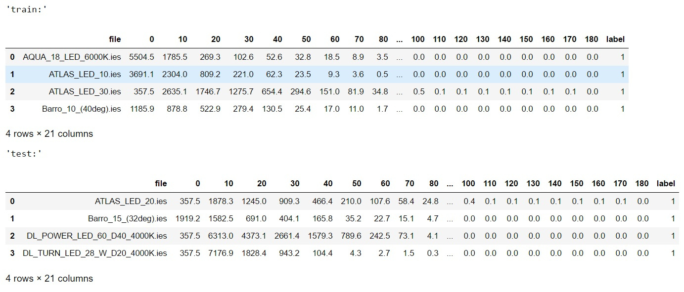
display('train:',train_df.head(4),'test:',test_df.head(4))
#divide the data and labels
X_train=np.array(train_df.iloc[:,1:-1])
X_test=np.array(test_df.iloc[:,1:-1])
y_train=np.array(train_df['label'])
y_test=np.array(test_df['label'])
���� �� ������ ���������� ������ ��� ������� � �������� ��������� �� python, �� ���� �������������� ��� ��� �� ���������� ��� ��� ���������.
�� �� ������ ������, � ������ �� ������� ������ �� ������� � �������� ������� � �������, � ����� �������� �� ��� ������� ���������� �������� (���� ����� � �������� �����) � ����� �������, �� � ������� �� ��� ����������� ����������� �� ������ 4 ������ �� �������, ��� ��� ����������:
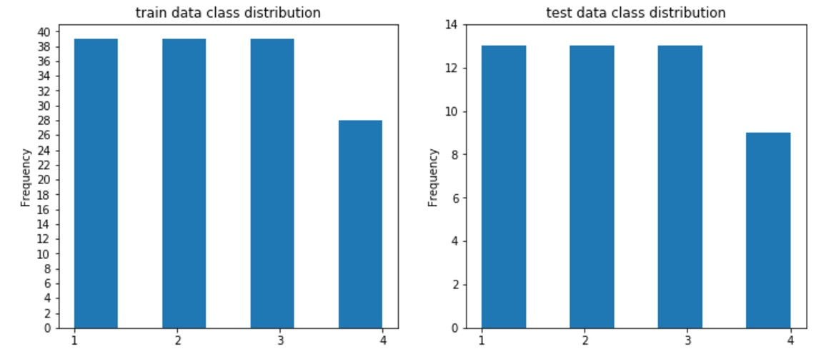
������ ��� �������� �� �����, ������ ����� ���� �������������� �� ���������� ������ �4( ������ �) � � ����� � ����� ��� ������ ���� ������� � ��� ����������� � 40 �������� � ������� ������� � 12 � �����������, ��� ������ � � 28 � ������� � 9 � ����������� � ����� ����������� ������� � 1/4 ����� ������� � ����������� �������� �����������.
�� � ���� �� �������� ������ �� ����� �� ������, �� ��������� ���:
#draw classdistributions

test_n_max=test_df.label.value_counts().max()
train_n_max=train_df.label.value_counts().max()

fig, axes = plt.subplots(nrows=1, ncols=2, figsize=(12,5))
train_df.label.plot.hist(ax=axes[0],title='train data class distribution', bins=7,yticks=np.arange(0,train_n_max+2,2), xticks=np.unique(train_df.label.values))
test_df.label.plot.hist(ax=axes[1],ti
� ������� ���������:
������� �������� � ����� ���������, ��� �� ��������� � ����� ������� ��� ��� �������� ���� � ���� ��������, �� ���� ����� ������ �� �� ��������� ���������� ����������� � ����������� ��������, � ������ ������� � ������� ��
�������� ���� , ����� � ��� ��� �������� ����� �������� ���� ������� ��������, � ���� ��� ��������� �������� ����� ��������� �������� ����� ������.
������� ������� ���������������� ��������. ������, ��� ������ ��������������� � scikit-learn ������ ������������ �� �������� (��� � �� ����������), � ��� ������������ �������������� �� �������� � ������ ������, ��� �� �������� �������� � ������ �����������, ��� ������� ��� ������� �
��������� ����������������� ������������� ��������!
�� � ���� ����� ������ ����� �������������� ������ �� �������� (�� �������), ����� ��������� �������� ������������� ��� ����� �� �����, �� ��� ���� ������� ���� ������� � �������� ����� 0 � 1.
��-�������� � ������, ��� � ����� ���� ����� �������������� ��������� ������� � ����������� ����� ������� (��������� �� ��������� �������), �� � ����� ������, ��� �� ��������� ��-�� ������������ ����� ��������� (� �������� ������� ������ ����� � ����������������� ������� ����� ����� ������ ��������), ������� �������� ������ ������� �� ������.
������� � �����, ������������� � ������ ������, � �������� ������������� � ������ ������� � ���� �� ���������.
#scaled all data for final prediction
scl=MinMaxScaler()
X_train_scl=scl.fit_transform(X_train.T).T
X_test_scl=scl.fit_transform(X_test.T).T

#scaled part of data for test
X_train_part, X_test_part, y_train_part, y_test_part = train_test_split(X_train, y_train, test_size=0.20, stratify=y_train, random_state=42)

scl=MinMaxScaler()
X_train_part_scl=scl.fit_transform(X_train_part.T).T
X_test_part_scl=scl.fit_transform(X_test_part.T).T
���� ���� �� ������ �������, �� �� ���� ������ �� ��������, ��� � ���� ������� �� ������ scikit-learn ������ ���������, �� ������� ������ ��������� ������ � ����� fit, ���� ��� ���� ���������������� ������, �� �������� ����� transform (� ����� ������ ���������� ����� 2 � 1), � ���� ���� ����� ����� ����������� ������ �������� ����� predict � ����������� ��� ���� ����� (�����������) �������.
�� � ��� 1 ��������� ������, ������� ����������, ��� � ��� ��� ����� ��� ����������� �������, ��������, �� ������ ������ �� kagle, ��� ��� ����� ������� �������� ������������ ������?
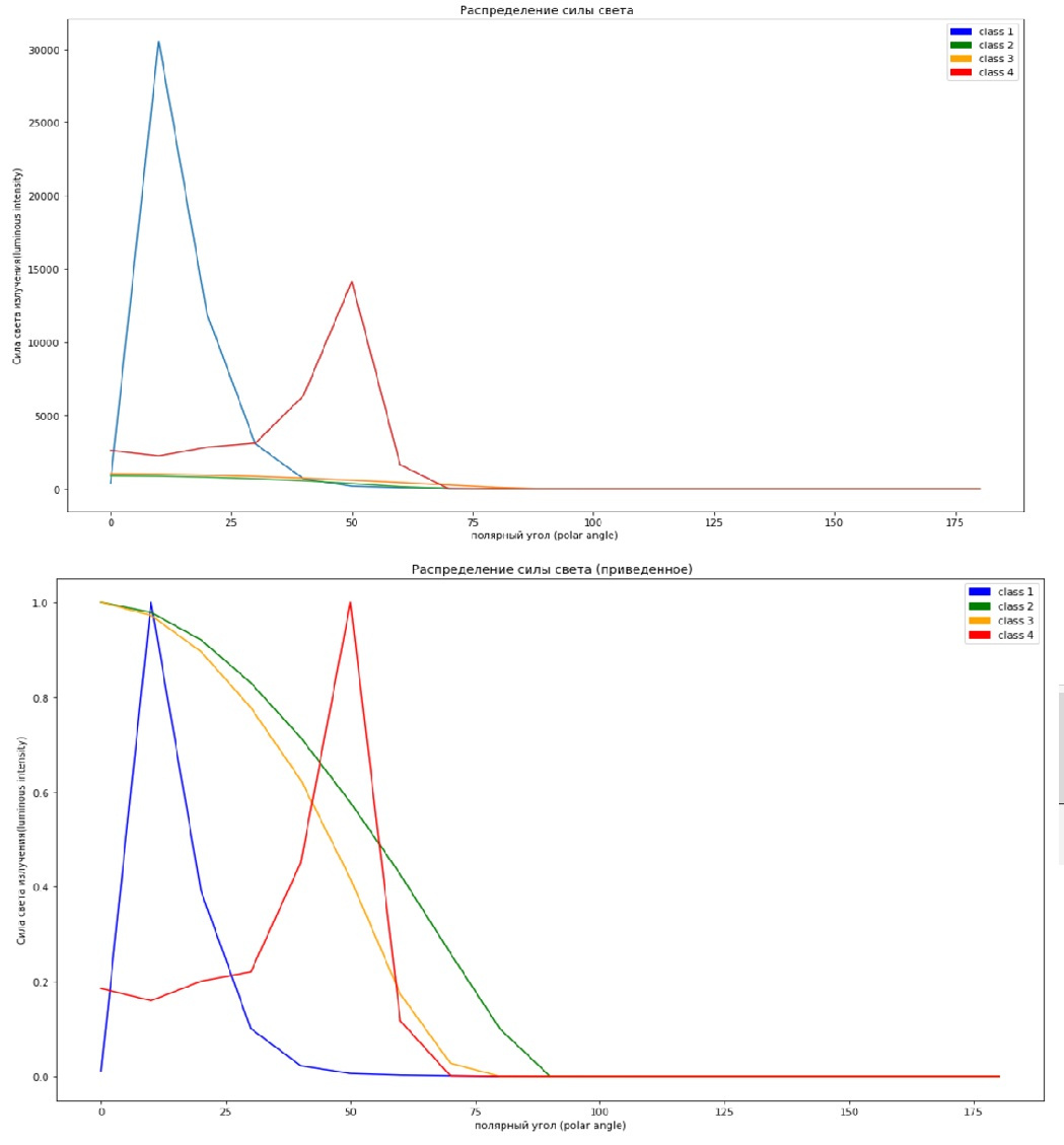
�����, ��� ������ ������, ��� �� ��������� ������� ������ ����� ����� �� ����� ������� �������� ����� �������� ��������� ������� �� ��� ���� ��������� (�� ��������) � �������� (�� ������� ���������), ��� ��� ���������� ���� �����. � ���� �������� � ��������������� � ���������, ��� ��� ��� �������, ������� �������� ��� ��������������� ���������, ������ � ����������������.
#not scaled
x=np.arange(0,190,10)
plt.figure(figsize=(17,10))
plt.plot(x,X_train[13])
plt.plot(x,X_train[109])
plt.plot(x,X_train[68])
plt.plot(x,X_train[127])
c1 = mpatches.Patch( color='blue', label='class 1')
c2 = mpatches.Patch( color='green', label='class 2')
c3 = mpatches.Patch(color='orange', label='class 3')
c4 = mpatches.Patch( color='red',label='class 4')
plt.legend(handles=[c1,c2,c3,c4])
plt.xlabel('�������� ���� (polar angle)')
plt.ylabel('���� ����� ���������(luminous intensity)')
plt.title(' ������������� ���� �����')
������� ��� � ������ ������ (�� ��� �������� subplot)
#scaled
x=np.arange(0,190,10)
plt.figure(figsize=(17,10))
plt.legend()
plt.plot(x,X_train_scl[13],color='blue')
plt.plot(x,X_train_scl[109],color='green')
plt.plot(x,X_train_scl[68], color='orange')
plt.plot(x,X_train_scl[127], color='red')
c1 = mpatches.Patch( color='blue', label='class 1')
c2 = mpatches.Patch( color='green', label='class 2')
c3 = mpatches.Patch(color='orange', label='class 3')
c4 = mpatches.Patch( color='red',label='class 4')
plt.legend(handles=[c1,c2,c3,c4])
plt.xlabel('�������� ���� (polar angle)')
plt.ylabel('���� ����� ���������(luminous intensity)')
plt.title(' ������������� ���� ����� (�����������)')
�� �������� �������� �� ������ ������� �� ������� ������ � ��� �� ����� � ��� � ���������� ����� ����� ���-�� ������ �� ����������������� �������, ��� �� ������� ��������� ������� ������ ��������� � ����� ��-�� ������� ���������.
��� ����, ����� ������������ �������� � ����� �������, ������� ��������� ������� ����������� ��������� �� ����������, ����� ���������� ���� ������ �� ���������� �������� � ���������� �� ������� ���� ������ ��������� (�� ������������� ��� ����� t-SNE)
����� ��� ��������������� ������ � ����������������
#T-SNE
colors = ["#190aff", "#0fff0f", "#ff641e" , "#ff3232"]
tsne = TSNE(random_state=42)
d_tsne = tsne.fit_transform(X_train)
plt.figure(figsize=(10, 10))
plt.xlim(d_tsne[:, 0].min(), d_tsne[:, 0].max() + 10)
plt.ylim(d_tsne[:, 1].min(), d_tsne[:, 1].max() + 10)
for i in range(len(X_train)):
# ������ ������, ��� ����� ������������ ��������� ������ �����
plt.text(d_tsne[i, 0], d_tsne[i, 1], str(y_train[i]),
color = colors[y_train[i]-1],
fontdict={'weight': 'bold', 'size': 10})
plt.xlabel("t-SNE feature 0")
plt.ylabel("t-SNE feature 1")
������� ��� � ������ ������ (�� ��� �������� subplot)
#T-SNE for scaled data
d_tsne = tsne.fit_transform(X_train_scl)
plt.figure(figsize=(10, 10))
plt.xlim(d_tsne[:, 0].min(), d_tsne[:, 0].max() + 10)
plt.ylim(d_tsne[:, 1].min(), d_tsne[:, 1].max() + 10)
for i in range(len(X_train_scl)):
# ������ ������, ��� ����� ������������ ��������� ������ �����
plt.text(d_tsne[i, 0], d_tsne[i, 1], str(y_train[i]),
color = colors[y_train[i]-1],
fontdict={'weight': 'bold', 'size': 10})
plt.xlabel("t-SNE feature 0")
plt.ylabel("t-SNE feature 1")
�������� �������, ������ ��� � ����� ����� ������ ����� �� � ����.
�� �������� �����, ��� �� ���������������� ������, ������ 1, 3, 4 ����� ����� ������ ���������, � ����� 2 �������� ����� �������� 1 � 3 (���� �� �������� � ���������� ��� ������������, �� �� ������� ��� ��� � ������ ����)
������
�� ��� �� ���� ��� ���������� � ���������������� �������������
��� ������ ������ SVC �� ����� ���������� �������
#predict part of full data (test labels the part of X_train)
#not scaled
svm = SVC(kernel= 'rbf', random_state=42 , gamma=2, C=1.1)
svm.fit (X_train_part, y_train_part)
pred=svm.predict(X_test_part)
print("\n not scaled: \n results (pred, real): \n",list(zip(pred,y_test_part)))
print('not scaled: accuracy = {}, f1-score= {}'.format( accuracy_score(y_test_part,pred), f1_score(y_test_part,pred, average='macro')))
#scaled
svm = SVC(kernel= 'rbf', random_state=42 , gamma=2, C=1.1)
svm.fit (X_train_part_scl, y_train_part)
pred=svm.predict(X_test_part_scl)
print("\n scaled: \n results (pred, real): \n",list(zip(pred,y_test_part)))
print('scaled: accuracy = {}, f1-score= {}'.format( accuracy_score(y_test_part,pred), f1_score(y_test_part,pred, average='macro')))
������� ��������� �����
�� ����������������
not scaled:
����������������
scaled:
��� ������ ������� ����� ��� �����������, ���� � ������ ������ ��� ������� �������
����������� ������ �������� ����� ��� ��������� ������������, �� �� ������ ������ �� �������� 100% ���������.
������ ���� ������ �� ������ ������ ������ � ��������, ��� � ��� ����� 100% ���������
#final predict full data
svm.fit (X_train_scl, y_train)
pred=svm.predict(X_test_scl)
print("\n results (pred, real): \n",list(zip(pred,y_test)))
print('scaled: accuracy = {}, f1-score= {}'.format( accuracy_score(y_test,pred), f1_score(y_test,pred, average='macro')))
��������� �� �����
results (pred, real):
��������! ���� ��������, ��� ������ � �������� accuracy � ����� ������������ f1-score, ������� ��� �� ����������� ���� �� ���� ������ ����� ����������� ������� ���������, � ��� � ����� ������ ������� ����� ��������� ����� ������� (�� ���� �� � ���� ��������� ��������)
�� � ���������, ��� �� � ���� �������� ��� ��� �������� ��� ������������� RandomForest
� ������ � � ������ ����������, � �����, ��� ��� RandomForest �� �������� ��������������� ���������, ��������� ��� �� ���.
rfc=RandomForestClassifier(random_state=42,n_jobs=-1, n_estimators=100)

rfc=rfc.fit(X_train, y_train)
rpred=rfc.predict(X_test)
print("\n not scaled: \n results (pred, real): \n",list(zip(rpred,y_test)))
print('not scaled: accuracy = {}, f1-score= {}'.format( accuracy_score(y_test,rpred), f1_score(y_test,rpred, average='macro')))


rfc=rfc.fit(X_train_scl, y_train)
rpred=rfc.predict(X_test_scl)
print("\n scaled: \n results (pred, real): \n",list(zip(rpred,y_test)))
print('scaled: accuracy = {}, f1-score= {}'.format( accuracy_score(y_test,rpred), f1_score(y_test,rpred, average='macro')))
������� ��������� �����:
not scaled:
����, ����� ������� 2 ����������:
1. ������ ������� �������������� �������� ���� ��� �������� ��������.
2. SVC ������� ������ ��������.
���� ��������, ��� � ���� ��� � ��������� �������� ������� � ���� ��� scv � �� ������ �� ����� �������� ������ �������, �� ��� Random Forest �� �������� � � 10-�� ����, ������ � ������� �� ��������� (�� ����������� ����� ��������). �������� ���� ���������, ������� ������� �������� �� 100%, ���������� ��������� � ����������� ���������� � ������������.
�� ��� ����� � ���, �� �����, ��� ������ �������� ����, ��� �� �������, ��� � �� �������� ������� ����� ����, �������
������
�������� �������� ���������, ��������� ������������� ������, � ��-�������� ������� ������� ����������� ��������� � ������ ������ ������� ������ ���.
�� � ���� ����� ���-�� �� ���������, �� �� ������� ��� ��� �� �������� �����.
��-��! ����� �� �� �������� ��� ������ ��� ����� ��� � ������� ������ ������� �������� ;)
� �� �������� � ���� ����!